Throughout your studies in Mathematical Methods, you learn about a lot of different types of graphs. In this article, we will look at how to sketch polynomial graphs.
The Study Design has explicitly stated 4 polynomial graphs you need to know about. These are all apart of Area of Study 1, titled ‘Functions, Relations, and Graphs.’
There’s so much involved in sketching a polynomial – from intercepts to turning points to point of inflections.
Keeping track of all the key features in polynomials can be quite overwhelming, so hopefully this article will make some things clearer and easier!
Before we begin, let’s recap the definition of a polynomial.
A polynomial is an expression that consists of variables and coefficients. Each term in a polynomial
expression is separated by either addition or subtraction. The variables are raised to a power, but the powers must be a natural number (a whole number that isn’t positive).

-
For example, 2x2+3 is a polynomial, but 5x1/2 is not. Can you work out why?
-
The polynomial functions that you need to be able to sketch are: y = x, y = x2, y = x3, and y = x4.
1. Linear graphs (y = x)
A linear graph is simply a straight line on a plane, where x is raised to the power of 1. You would have studied linear graphs in previous years, so most of these points should be revision for you.
Linear graphs have 3 key features:
- x intercept
- y-intercept
- Gradient
The general form of a linear equation is as follows:

The gradient of a line refers to how steep it is – the larger the gradient the steeper the line.
Gradients can also be positive or negative. One way to remember the difference is that:
-
Positive gradients slope upwards – it’s like climbing up a hill.
-
Negative gradients slope downwards – it’s like climbing down a hill.
To sketch a linear graph, simply find the x and y-intercepts, locate them on the axis and draw a nice straight line joining the two points together. Remember, to find the x-intercept, let y equal 0 and rearrange the equation to find x. To find the y-intercept, you can simply read off the number added/subtracted on the end of the equation.
Here's the graph of y = –2x+6:
Keen to learn more about linear graphs? Check out this video: https://www.youtube.com/watch?v=XlacofDkPGs
2. Quadratic graphs, aka parabolas! (y = x2)
Parabolas will be the type of graph that you will study the most in Year 11. The main feature of a parabola is its turning point. A turning point is a point on a graph where the graph switches from increasing to decreasing. Quadratic graphs also have up to two x-intercepts and a y-intercept.
These graphs are perfectly symmetrical – the turning point occurs right at the mid-point of the curve.
This is the graph of y = x2, it has a turning point and intercept at (0,0):
We can also shift this graph across the plane and do lots of fun transformations to it.
Let’s look at the equation (x–2)2–16. This equation is in turning point form – you would have learnt about this in your studies of algebra.
This graph has a turning point at (2,–16). If you solve for the intercepts, you’ll find that they are at (0,–12), (–2,0), and (6,0).
To sketch it out, simply locate the intercepts and turning point on the graph and draw a smooth line connecting all the points. 
You can also sketch quadratics when they’re in factorised form: y = a(x–b)(x–c). To do this, you can apply the null factor law to find the x-intercepts, locate the turning point and once again, draw a line through all the points.
Do you remember what happens when there is a negative sign in front of the equation? What happens to the turning point?
Cubic graphs (x3)
Cubics are polynomials where x is raised to the power of 3. Before setting out to graph these, you should have learnt a variety of different techniques to help factorise them, such as the factor theorem, remainder theorem and long division.
The graph of y = x3 looks like this: 
There is a point of inflection, and intercept at (0,0). A point of inflection is a flat point in the graph, and it is where the function changes concavity. If you were to transform this exact graph in the plane, the equation would take on the form y = a(x–h)3+k, where the point of inflection is at (h,k).
A cubic graph with its equation in factorised form has up to 3 x-intercepts and 2 turning points. You will not be required to know how to find the coordinates of the turning points until you learn calculus in Unit 2. Phew! Once again, when the equation is in factorised form, simply apply the null factor law to find the x-intercepts, solve for the y-intercept then connect everything together.
Here’s the graph of y = (x–3)(x+2)(x–1).

4. Quartic Graphs (x4)
Like cubic graphs, quartic graphs are a new type of graph you will encounter this year. Students tend to forget their existence and get quite surprised when they appear on tests and exams!
At first glance, they do look quite like a quadratic graph. The general graph of a quartic (y = x4) looks like this:

As you can see, the graph has a turning point (and intercept) at (0,0). Unlike in a quadratic, the turning point is much flatter. When you sketch out a quartic, you must remember to flatten off the turning point, otherwise your teacher might think you sketched a quadratic instead!
Quartics can also be translated and rewritten in the form y = a(x–h)4+k. The way to sketch out a quartic in this form is identical to the way you would do a quadratic.
Just like in cubic and quadratics, you can sketch quartics when the equation is in factorised form. There will be up to four x-intercepts, a y-intercept and three turning points.
Simply apply the null factor law to find the x-intercepts, and the algebraic method to find the y intercept. Connect all those points with a turning point in between two intercepts. Also pay attention to any negative signs that are present in the equation, as this will change the way the graph is oriented.
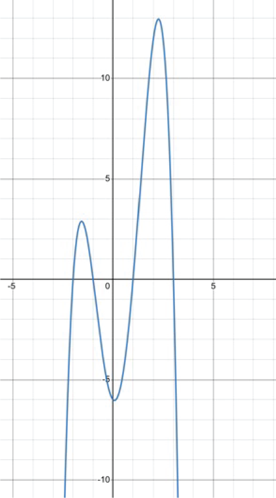
Graph of a positive quartic: (x–1)(x+2)(x–3)(x+1)

Graph of a negative quartic: –(x–1)(x+2)(x–3)(x+1)
Some general tips for sketching polynomials
-
Make sure all intercepts, turning points and points of inflection are labelled with the correct coordinates.
-
Draw a smooth line connecting all the points – marks will be lost if the graph looks sketchy!
-
Any coordinates should be labelled with the numbers in exact form (i.e. no decimals) unless otherwise specified.
That brings us to the end of polynomial graphs. Hopefully you didn’t find this all too bad! These graphs will come up time and time again in Methods, and it is important that you get a good hang of sketching them. These graphing techniques, combined with algebra, lead itself to some difficult problem solving type questions, so by getting the hang of these basics, you will really set yourself up for success!
In case you want do delve into this topic more deeply, have a look at these free notes.