The Normal Distribution (aka Gaussian Distribution) is an extremely useful tool that statisticians use to model situations that involve a continuous random variable. Just like any probability distribution, it describes how the values of a variable are distributed (we’ll get more into this later). However, statisticians use this distribution more than others, as it describes the distributions of natural phenomena very accurately.

In your studies of statistics, you will learn about the characteristics of the normal distribution, and how to do calculations based on it. This article will go through some of these, so hopefully you will leave feeling a lot more confident with this concept!

The Normal Distribution

Before we learn about the characteristics of the Normal Distribution, we need to understand what a probability density function is.

This is a statistical function that describes the likelihood of obtaining all possible values that a random variable can take. In simple terms, it tells us the probability of something occurring.

Have a look at the arbitrary probability density function below.

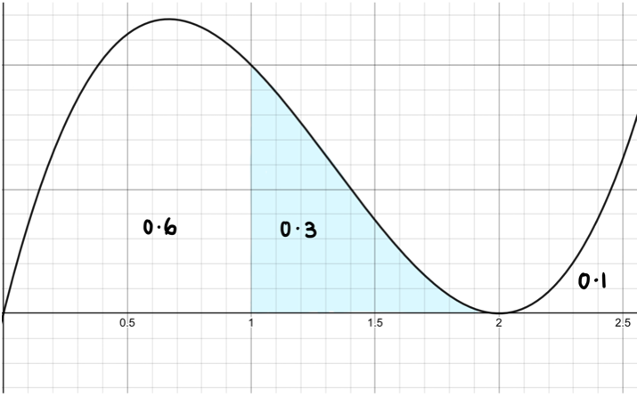
The area under the curve represents the probability and corresponds to the numbers (aka observed values) on the x-axis. In this case, the probability of being between 1 and 2 is 0.3.

The normal distribution is a special type of probability distribution function, and is described by the following equation: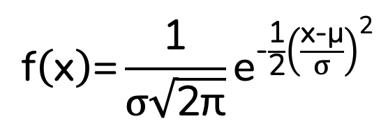

Where:

x = value of the variable or data being examined
μ = the mean
σ = the standard deviation

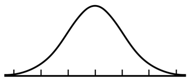
The general shape of the graph is called a ‘bell curve.’

As you’d expect, the normal distribution has some key characteristics, that makes it different from other probability density functions.

The data is perfectly symmetrical around the mean. As such, the probability of getting a value below the mean or above the mean is 0.5. The mean is in the centre of the graph.
The mean, median and mode are all equal.
The total area under the curve is 1, as probabilities can never exceed 1. As discussed above, the area under the curve between x values give the probability of them occurring.
The graph asymptotes along the horizontal axis.

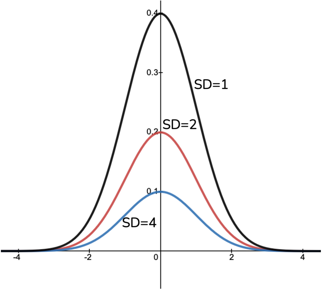
The general shape of the distribution is always the same, but the value of the standard deviation and mean changes its proportions. The standard deviation is a measure of the spread of the data and corresponds to the width of the graph. The larger the standard deviation, the flatter the graph will be.

You can see this in the diagram below.

Changing the mean will just change the position of the graph on the horizontal axis – the actual graph doesn’t change.

Z-Scores

A special type of normal distribution is called the ‘standard normal distribution,’ or the ‘z distribution.’ This refers to the special case where the mean is 0 and the standard deviation is 1.

Since the standard deviation is 1, you can easily see how far away you are from the mean. For example, if you had an x-value of 5, you can easily work out that you are five standard deviations away from the mean.

However, it goes without saying that the scenarios you will be working will not have a mean of 0 and SD of 1. Therefore, it is handy to convert the values you must something called a ‘z-score,’ which relates to the standard normal distribution. This process is called standardization, and the formula to do so is as follows:

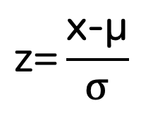
Where:

z=corresponding z score
x=value being converted to a z score
μ = the mean of the original distribution
σ = the standard deviation of the original distribution

The z-score will tell you how many standard deviations you are away from the mean for any given x-value.

The 68-95-99.7% Rule

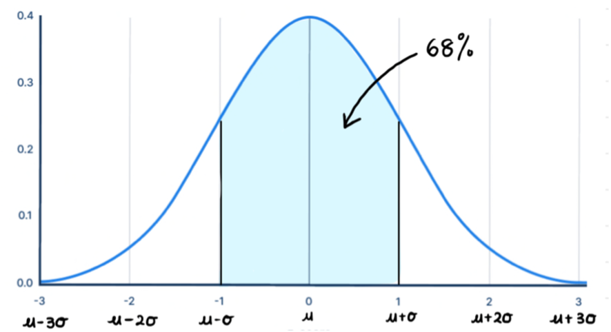
A handy rule that is used when analysing normal distributions is called the 68-95-99.7% rule. This rule tells us the area under the curve between standard deviations.

68% of the data lies between one standard deviation of the mean. The combined area in the tails is 32%, so each tail has 16% of area.

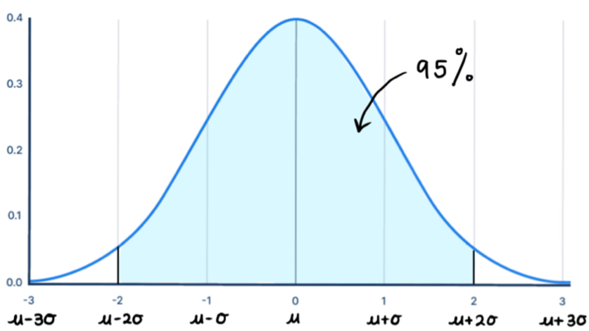
95% of the data lies between two standard deviations of the mean. The combined area in the tails is 5%, which means each tail has 2.5% of area.
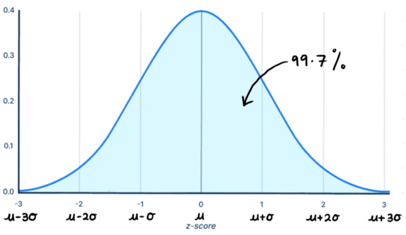
99.7% of the data lies between three standard deviations of the mean (which is almost all of it!). The combined area is the tails is 0.3%.

Example

Let’s do an example to summarise what was covered in this article.

The average age of people in a workplace was normally distributed with a mean of 22.3 and a standard deviation of 2.6.

a) What is the probability of randomly selecting a person that is between the ages of 17.1 and 27.5?

First, we need to convert the given values into z-scores.

z1=(17.1-22.3)/(2.6)=-2

z2=(27.5-22.3)/2.6=+2

We can see that we are between 2 standard deviations of the mean, which corresponds to an area of 0.95. Therefore, there is a 95% chance of randomly selecting a person between those two ages.

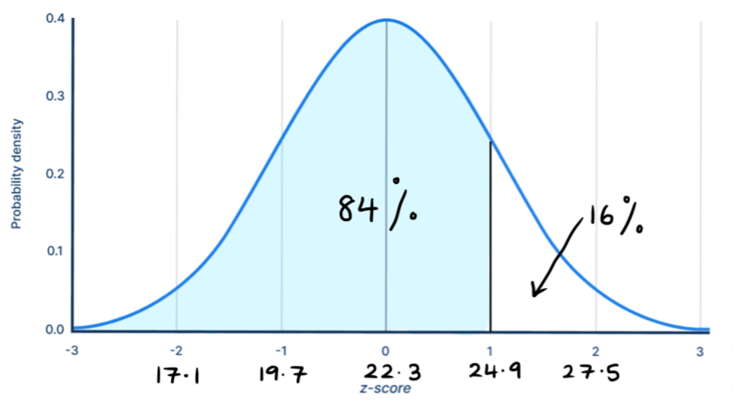
b) What is the probability of randomly choosing a person who is under the age of 24.9?

Once again, we’ll convert this into a z-score.

z=(24.9-22.3)/2.6=+1

This value is one standard deviation to the right of the mean. The area between 1 standard deviation on either side of the mean is 68%, which means the area to the right of this value is 16%. The area to the left of this value is what we are after, since we want the people younger than 24.9. Since the total area is 1, we can subtract 16% from it.

Thus, the probability of randomly selecting a person less than 24.9 years is 84%.

Hopefully this article helped you gain a better understanding of the normal distribution. You should make it a point to understand the theory behind it before jumping into practise questions. It will definitely come up in your tests and exams!

You can download a set of summary notes for this topic here.